Understanding Bootstrapping: A Key Statistical Technique
Written on
Chapter 1: Introduction to Bootstrapping
If you're engaged with substantial datasets, the concept of bootstrapping is likely familiar to you. For those stepping into the fields of statistics or bioinformatics, it’s a crucial tool in your analytical arsenal. But what exactly does bootstrapping entail, and why is it significant?
Bradley Efron introduced bootstrapping in 1979, and this computationally intensive method gained traction as computing resources became more accessible. Notably, the bootstrapping technique has been referenced over 20,000 times in research literature.
When analyzing large datasets, our goal is to derive insights about the population from which our data originates. Although we can compute metrics like the mean or median, the reliability of these estimates remains uncertain. Increasing our sample size can enhance accuracy, but this isn't always feasible, especially in cases like RNA sequencing or extensive data collection, where the costs can be prohibitive. Bootstrapping serves as a resampling technique that allows us to estimate errors and confidence intervals. The insights gleaned from bootstrapping can influence conclusions across various applications, including financial data analysis, phylogenetic studies, and gene expression assessments.
Defining Bootstrapping
Bootstrapping is essentially a method of resampling with replacement. To clarify how this works, let's explore an illustrative example along with the fundamental assumptions involved.
Imagine we have a dataset representing the fees charged by basketball players for birthday appearances. However, due to limitations, you've only managed to contact eight players, making your dataset, D, contain just eight values. Your sampling includes a diverse group of players to ensure that the sample reflects the broader population.
This leads us to a statistical assumption: our sample effectively represents the population distribution.
D = {100, 200, 200, 300, 500, 1000, 1000, 750}
In this scenario, the average of our sample D is 506.25. By bootstrapping this sample multiple times, we can gain insights into the variance within the data. The bootstrapping process involves resampling with replacement. Each resampled bootstrap will consist of eight values, and because of the replacement, certain values (for instance, 100) might appear more than once. Consequently, bootstrapping can yield varying estimates with each iteration. However, with a sufficient number of bootstraps, we can approximate the data's variance.
It's important to note:
- We aren't introducing any new data points into our dataset.
- Each resampled bootstrap retains the same number of values as the original sample.
- The probability of selecting any particular value remains constant across the bootstrap process. For example, if the first resampled value is 200, it doesn’t affect the likelihood of the next selection also being 200.
Here are some example bootstrapped samples:
D? = {100, 1000, 500, 300, 200, 200, 200, 100}
D? = {300, 1000, 1000, 300, 500, 100, 200, 750}
D? = {750, 300, 200, 200, 100, 300, 750, 1000}
The averages of these samples, D?, D?, and D?, are 325, 518.75, and 450, respectively. These values can then be utilized to derive the standard error, confidence intervals, and other relevant metrics. Utilizing programming languages like Python or R, you can easily generate 50, 100, or even 1000 bootstrapped samples. Understanding the bias, variance, and distribution of your sample enhances the accuracy of your inferences regarding the population it represents.
While this example uses a small dataset, it's worth noting that bootstrapping is generally not suitable for small datasets, those with significant outliers, or those involving dependent measures.
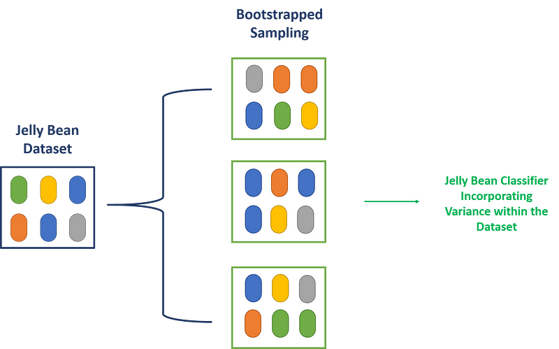
To further illustrate bootstrapping, I have included a visual representation using a jellybean dataset.

Chapter 2: Applications of Bootstrapping in Bioinformatics
The first video, "Why 'Pulling Yourself Up by Your Bootstraps' is Bad Advice," delves into the misconceptions surrounding bootstrapping, providing context for its application in statistics.
The second video, "You're Using 'Pull Yourself Up By Your Bootstraps' Wrong," further clarifies common misunderstandings about the technique and its proper uses.
Example 1: Phylogenetic Trees
Bootstrapping is instrumental in evaluating the confidence of branches within a phylogenetic tree. By resampling an amino acid sequence or a nucleotide sequence from a gene, we can quickly create 1,000 bootstrapped trees. If your original tree indicates a specific protein or gene sequence branching off, you can examine the bootstrapped trees to see the frequency of this branch's occurrence. If it appears over 950 times, you can be reasonably confident in the robustness of your data. Conversely, if it only appears around 400 times, it may be due to an outlier.
Example 2: Estimating Gene Transcript Abundance
The Sleuth software employs a bootstrap methodology to estimate gene transcript abundance. By resampling next-generation sequencing reads, we can derive a more accurate estimation of transcript levels. This resampling captures the technical variability in the data, which, when combined with biological variability, helps determine if a specific gene or transcript is significantly elevated in your dataset.
Other Applications of Bootstrapping
Bootstrapping is also applied in ensemble machine learning, where datasets are resampled multiple times. Each bootstrapped sample is processed through a classifier or machine learning model. By aggregating the results, we can achieve a more precise classifier, reducing the risk of overfitting the data based on a limited sample.