Chapter 1: Understanding Turbulence and Financial Markets

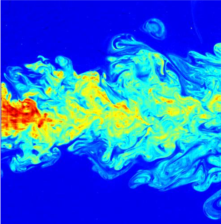
There are intriguing parallels between the dynamics of turbulent fluids and financial markets. In both scenarios, significant disturbances propagate through progressively smaller scales (refer to the works of Stanley and Mantegna). When you stir a liquid, you can observe how the energy introduced into the system transitions to smaller scales. Similarly, in financial markets, information is disseminated on a grand scale, resulting in reactions that affect individual investors at smaller scales. Modeling both phenomena is complex due to the diverse types of interactions present among their components or in relation to their environments.

Here, we will demonstrate, supported by a comprehensive statistical analysis by Stanley and Mantegna, that while there are qualitative similarities between financial markets and turbulent fluids, the quantitative parallels are limited.

What is Turbulence?

Consider a fluid flowing through a pipe characterized by the following parameters:

• Kinematic viscosity (ν): This is also known as momentum diffusivity and is defined as the ratio of the viscosity (η) to the fluid's density (ρ).
• Velocity (V)
• Pipe diameter (L)

In fluid mechanics, the Reynolds number (Re) is a crucial dimensionless metric that predicts flow patterns. The Reynolds number for the flowing fluid, based on the parameters specified, can be expressed as follows:

The value of Re indicates the complexity of the fluid. Depending on its value, the fluid may exhibit either turbulent (high complexity) or laminar (low complexity) behavior. The transition from laminar to turbulent flow is termed laminar-turbulent transition.

The Navier-Stokes equations, which define the dynamics of incompressible fluids, are given by:

where V(r,t) denotes the velocity vector field and P represents pressure. Equation 2 describes turbulent regimes characterized by very high Re (fully developed turbulence).

Energy Cascades in Turbulence

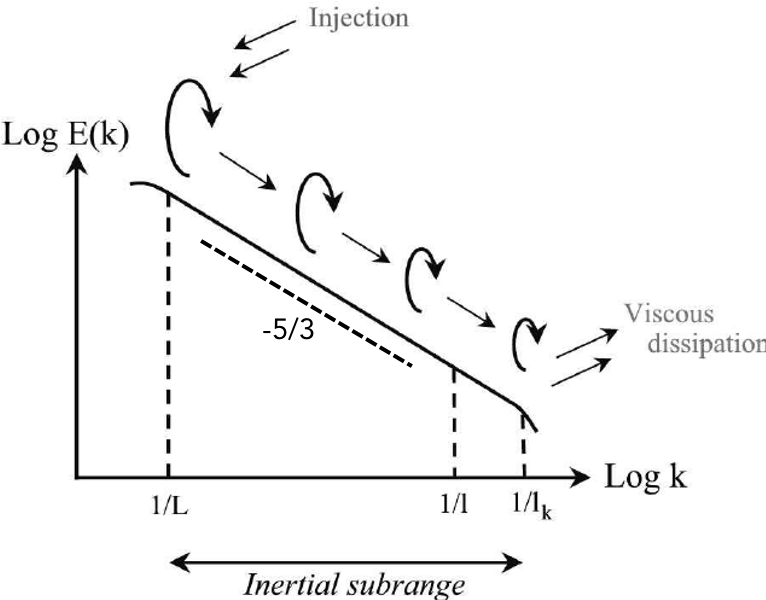
In systems exhibiting nonlinear dynamics, such as a fluid in a turbulent state, energy may undergo direct (or inverse) cascades, transferring energy between large and small scales of motion. If intermediate scales are present, this range is referred to as the inertial range.

The energy spectrum within the inertial range typically follows a power-law distribution:

Kolmogorov's 1941 Theory

The esteemed mathematician Andrey Kolmogorov demonstrated that for fluids with fully developed turbulence (as Re approaches infinity), the following behaviors are observed:

This equation describes the mean square velocity increment in the inertial range. However, Kolmogorov's theory does not account for the intermittent behavior observed in velocity changes, which leads to a leptokurtic distribution of U(t).

Comparing Financial Markets and Turbulent Dynamics

To evaluate the temporal characteristics of financial markets against turbulent fluids, Stanley and Mantegna assessed two primary quantities: the dynamics of the S&P 500 index from 1984 to 1989 and the velocity V(t) of a fully turbulent fluid with a high Re, specifically the wind velocity in the atmospheric surface layer above a canopy in Connecticut.

Short-term observations reveal that both processes are nonstationary, non-Gaussian, and exhibit intermittent behavior. In contrast, long-term observations show that both processes tend toward asymptotic stationarity.

Stanley and Mantegna conducted a series of four comparisons between the S&P 500 index and fluid velocity, focusing on:

1. Their time evolutions Y(t) and V(t)
2. Their variations Z(t) and U(t)
3. The standard deviations σ(Δt) for Z(t) and U(t)
4. The power spectra S(f) of both Y(t) and V(t)

Time Evolution of the S&P 500 Index and Fluid Velocity

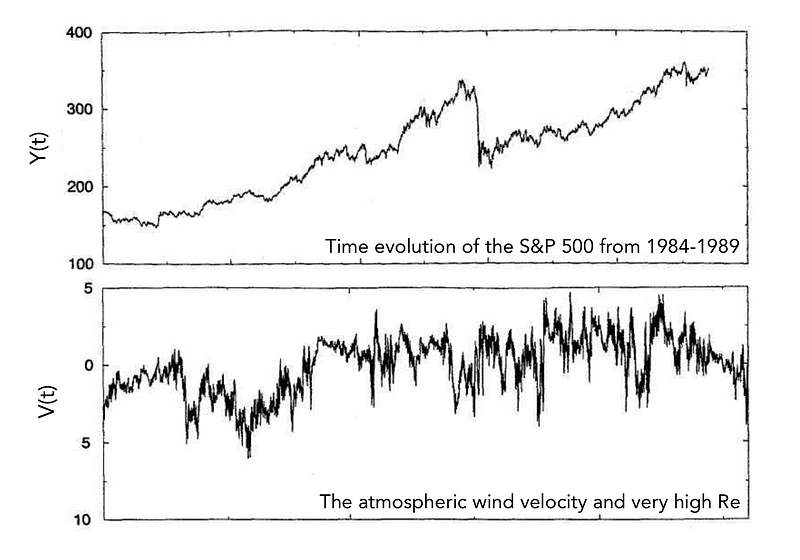
The following figure illustrates the time evolution of the S&P 500 index sampled at hourly intervals, alongside the atmospheric wind velocity during fully developed turbulence.

Changes in the S&P 500 Index and Fluid Velocity

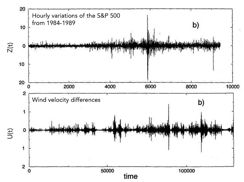
The subsequent figure presents the changes in the S&P 500 index over one-hour intervals compared to variations in fluid velocity (sampled at a higher frequency). Notably, the turbulent fluid displays symmetry about the x-axis, a characteristic absent in the financial data.

Standard Deviations of Increments in Financial and Fluid Dynamics

In their analysis, Stanley and Mantegna examined the volatility σ(Δt) for both processes Z(t) and U(t). Both processes exhibited power-law behavior, although the correlation of time between them differed significantly.

Spectral Densities and Their Analysis

The power spectrum of a stationary random process is determined through the Fourier transform of its autocorrelation function:

The spectral density of a random walk has a specific functional form:

Both processes can be compared through their power spectra, revealing a similar functional form, though with notable differences in their exponents.

Similarities and Differences in Dynamics

The comparative study of turbulent fluid dynamics and the S&P 500 index suggests that analogous methods can be utilized to analyze various systems governed by known yet unsolvable equations of motion.

Similarities include the presence of intermittent behavior and non-Gaussian probability distributions that gradually converge to a Gaussian attractor. Contrastingly, differences manifest in the shapes of the probability distributions and the correlation behavior of velocity fluctuations versus the S&P 500 index fluctuations.

This article derives insights from the discourse on the relationships between financial market dynamics and turbulent behavior as presented in a Nature Magazine article, alongside the foundational concepts outlined in H.E. Stanley and R.N. Mantegna's textbook.

For additional content covering finance, mathematics, data science, and physics, visit my personal website at www.marcotavora.me.