Chapter 1: Introduction to Linear Regression

Have you ever considered how mathematical concepts, particularly geometry, can shed light on data trends? In this article, we will explore linear regression as a method for understanding relationships among variables, utilizing various geometric principles. While terms like "vector calculus" may seem daunting, I assure you that the explanation will remain accessible. If you're intrigued by how shapes and lines can narrate data stories, let's embark on this journey.

In its simplest form, linear regression helps identify a set of vectors that best illustrate the overall trend within a dataset. This discussion aims to clarify the mathematical framework that underpins linear regression. We can express the variable set using the characteristic equation of linear regression: Y = I.P, where Y represents observations, I denotes input features, and P signifies the parameters vector.

Chapter 2: Loss Function and Its Significance

To minimize the difference between observed and predicted values, we define a loss function. The least squares loss can be expressed as L(e) = ||e||², where e = Y — I.P. To find the optimal parameters vector, we need to minimize L(e). Before diving deeper, let's analyze the geometric implications of this loss function. When does the loss reach its minimum?

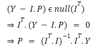
The defined loss is min(L(e)) = min ||Y — I.P||, and the vector Y — I.P is orthogonal to the column space of I, which corresponds to the null space of I. To clarify orthogonality, visualize the vector space of I.P; we are determining the distance (or loss) between the observation vector Y and the actual prediction derived from input features and the parameters vector I.P. This distance can be calculated element-wise as Y - I.P. Imagine a line extending from a point in the observation vector space, Y, to a corresponding point in the I.P vector space. The distance will be minimized when the distance vector is perpendicular to the vector space of I.P, thus confirming that the distance vector Y - I.P must be orthogonal to the column space of I. Remember, every vector that is orthogonal to a vector space resides within the null space of that space.

Chapter 3: The Calculus Approach to Minimization

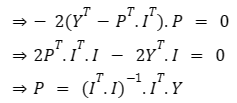
To minimize a function, we set the gradient to zero.

By equating the gradient of the loss concerning the parameters vector to zero, we can find the optimal solution.

Chapter 4: Implementation of Linear Regression

Here’s a simple implementation of linear regression using NumPy:

import numpy as np

def linear_regression(input_features, outputs):

'''

Arguments:

input_features (I): the feature matrix of the input data

outputs (Y): the observations or the output vector for input data

Returns:

matD: parameters vector

'''

# Using the derived formula from the discussion

matA = np.matmul(np.transpose(input_features), input_features)

matB = np.linalg.inv(matA)

matC = np.matmul(matB, np.transpose(input_features))

matD = np.matmul(matC, outputs)

return matD

I = [[1, 1], [1, 2], [1, 3], [1, 4]]

Y = [[2], [4.2], [6.1], [7.9]]

print(linear_regression(I, Y))

You can alternatively write your Python scripts for matrix operations without NumPy to achieve similar results.

Chapter 5: Conclusion

In conclusion, the integration of mathematical principles enriches our understanding of complex concepts, exemplified through linear regression. Utilizing analytical geometry to determine optimal parameters provides a vivid insight into the vector space of datasets. While this article presented a straightforward example of single-variable linear regression, the same techniques can be applied to multi-variable scenarios. Ultimately, it revolves around effectively navigating vector calculus and matrix transformations.

The first video titled "Lines and Parabolas I | Arithmetic and Geometry Math Foundations 73 | N J Wildberger" delves into the foundational concepts of geometry and its connection to data analysis.

The second video, "Calculus and Affine Geometry of the Magical Parabola | Algebraic Calc and dCB Curves 3 | Wild Egg," explores advanced topics in calculus and geometry that relate to regression analysis and data interpretation.

~Ashutosh